Chapter 1: What is it basically about?

Every software developer asks themselves the question at some point in their career: Why didn't I listen to my mother and become a doctor? Unfortunately, only the university place allocation department can tell you this, but for all other questions about determining error thresholds, this blog post should be useful to you or at least points out the right direction. So if you are currently developing a diagnosis f.e. that should help you detect upcoming errors in your software, then the choice of a suitable threshold is very important. This also applies to timeouts, safety functions and various other functions.
There are certain things that can go wrong. If you select a threshold value which is too close to the exact value of your system (without any tolerance) then you can easily get a “false failure”, an non-justified error. Or you choose the error value too generously and you don't get an error even if your system is already exceeding their limits. This is called a “false pass”. Both will lead to customer complaints in future, as either an unjustified error is constantly being reported to the customer or, in the worst case, an unrecognized error is harming your device. Both should be avoided equally. For better understanding, I used a real example from one of my recent projects.

Chapter 2: An example

Let's take a Modbus communication between a client and a server. The principle is quite simple, for example the client requests the value of a register from the server and receives an answer. This is exactly what we would expect under normal circumstances. But what if the server responds too late or not at all? Or the more important question, what does our system do? Our code would usually wait for a receive interrupt or an implemented timeout would exit our function at a maximum waiting time. Without this time it is a little bit like waiting for Godot and I can summarize the novel for you. He never showed up. Without a timeout, our system would be stuck in an endless loop waiting for an appropriate response. Well, I think you have understood the principle of the timeout. But how long are we willing to wait? Many will say at this point, “Take 1 second as a timeout” this is best practice. This value is based on experience, but it should be kept in mind that the timeout is hardly connected to your system behavior can vary depending on the system.

And what if we can't find a valid timeout value on Reddit or StackOverflow? Where do we start? Is 42 a good choice? Long story short. A test setup is needed. Once I measure a trace I can calculate the time between request and response which is in my case around 30 ms. Good then our line of code should be something like:

          handle_modbusTimeout_timer = xTimerCreate( "modbus_timeout", \
                                        pdMS_TO_TICKS(30), pdTRUE,     \
                                        (void*)0, timeout_cb  );       \
        

If we simply do it like that we will face some customer complaints in the future. What should we do instead? You have to examine the system in different states, ideally in a long-term test. A durability test run. One key element is that you measure all possible states of your system. Evaluating all the different noises which influence your system behavior is the hardest part. The rest is simply math and some lines of code. Let me show you an example. In our case we identify two main states of your server device:

Normal operation

Stress operation

Normal operation is representing your system under normal conditions. Stress operation, on the other hand, places a peak load on the system, especially the CPU, so that some tasks will be delayed. The main purpose here is to delay the response task of our server device in a way that we can better estimate what could be the worst case condition of the system. The whole thing represents a type of data collection under changing system conditions. Please keep in mind that this is only a very limited perspective, but completely sufficient for our example.

Chapter 3: The data collection

In the following chapter we take care about the data collection, but first we need some basic information about what it's all about. Data collection is the process of systematically collecting, recording, and organizing information to be used in analysis, reporting, or decision-making. It can take various forms, including manual entry, automated sensors, surveys, or digital data storage. The quality of data collection is crucial as it forms the basis for accurate analysis and technical decisions. In today's data-driven world, data collection plays a central role in areas of research and enables trends to be identified and processes to be optimized. Completely in our spirit.

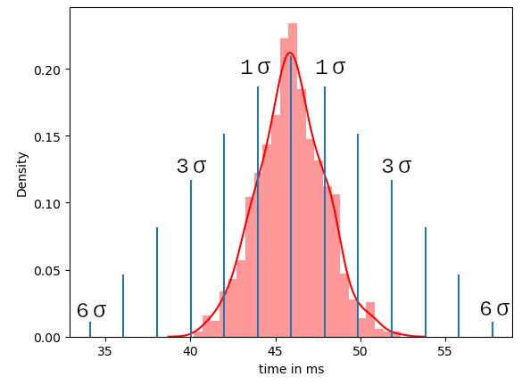
Let's get back to our example. We need to measure the delta between client request and server response to better understand how long a response takes. For better differentiation, we split the data collection into two individual measurements. The first data collected shows the response time under normal conditions. We then record a second series of measurements with a simulated stress operation in which we reprioritize some threads on the server device and add cpu intensive calculations. For those of you who do not have access to the server source code Interrupts are also quite suitable to stress the cpu..Or you can try to simulate a high data load on another communication interface by sending a large amount of data via the another interface. There are tons of different approaches to stress a system, which unfortunately I cannot fully address in this article. But just as a hint there are numerous software tools on the market which can help you to utilize system capacity. But sometimes. There are various options available.

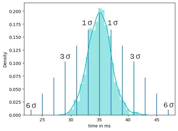
The following trace shows you an example how the device behaves under normal conditions. For the measurement I use a CH340 usb adapter and a self-written trace tool, which works quite easily under Linux and calculates the time delta at the same time if the header of the message is a duplicate the previous one. Are you using Windows or Mac? There are tons of good analysis tools available for free. Since the formatting of these tools always varies quite a bit, it is a good idea to post-process the data before further analysis. I do not cover this point in this article but you can reach out to me in case you need some assistance.

Side Note:
I personally work a lot with the python package “pandas”. This makes it easy to analyze the data series with a little practice. The data used here looks like this:

        13:24:02:4162, 0x03 0x02 0x00 0xc4 0x00 0x16 0xba 0xa9 || CRC: correct
        13:24:02:4483, 0x03 0x02 0x03 0xac 0xbd 0x35 0x20 0x18 || CRC: correct  
        >> delta 32,1 ms
        
         

You can save the follwowing data *.csv file and do the same calcaulation with the function shown in chapter 4

            30.5,34.4,32.9,32.0,36.5,34.1
           ,35.5,35.2,35.0,33.7,35.4,33.4
           ,34.9,37.9,33.7,33.9,34.1,35.3
           ,35.0,35.8,33.8,34.8,30.3,38.8
           ,34.6,32.9,34.8,33.3,35.3,30.9
           ,36.2,35.0,30.2,36.6,39.5,33.3
           ,35.0,38.6,33.6,33.7,33.9,37.0
           ,37.8,32.9,37.8,33.7,35.0,32.8
           ,37.9,35.1,35.9,35.9,34.8,37.7
           ,32.7,33.0,36.2,35.9,30.6,33.5
           ,34.4,32.4,35.4,37.6,35.4,34.6
         
          

Chapter 4: With the help of Python

For further evaluation we need the following python packages:

matplotlib - for the mathematical plots

seaborn - statistical data visualization

You can easily install both packages using the pip install command as follows:

          pip install matplotlib
          pip install seaborn
         

We then read in the data and can calculate the histogram and the Gauß normal distribution. As explained in the previous chapter, we should evaluate the two measurements one after the other. My recorded data is stored in a *.csv file format and can be read and processed with the following code example. If you would like to use pandas you only have to make some small adjustments.

          import csv
          import numpy as np
          import matplotlib.pyplot as plt
          import seaborn as sns
          
          x = [] 
          
          with open('2024-10-8_Modbus_measurement_normal.csv', mode='r') as file:
              filtered = (line.replace('\n', '') for line in file)
                  
              for line in filtered:
                output_fromFile = line.split(",")
                
                for elements in output_fromFile:
                  if (elements != ''):
                    x.append(float(elements))
          
          sns.histplot(x, kde=True, color='c', fill=True, stat="density")
          plt.show()    
                  
                

After we have read the csv data and removed unnecessary line breaks and spaces, we use the function histoplot(), which visualizes the corresponding histogram including the normal distribution curve. For simplicity, your histogram will be output without the sigma hyphens. To get also the sigma hyphens you need to add the following lines of code to your program:

          deviation = np.std(x)
          average = np.mean(x)

          for i in range(1,7):
            plt.axvline(x=(average - (i*deviation)), ymin=0, ymax=(0.9 - (i/7)))
            plt.axvline(x=(average + (i*deviation)), ymin=0, ymax=(0.9 - (i/7)))

          plt.axvline(x=(average), ymin=0, ymax=(0.85))
          
        

Lets review the histogram and see what details are in there. From the histogram we can see that the mean is around 35.03 ms and the standard deviation is 1.997. If we now go 6-sigma to the right in direction of the positive x-axis, our threshold is 47.02 ms. So the probability that a random value is in the range from -6-sigma to +6-sigma would be 99.9998%. Sounds pretty safe, especially since we don't want to cover the area in the negative direction for our timeout. Faster can also lead to errors, but this is not relevant in our given case. So let's note down 47.02 ms and set a timer of 50 ms for our timeout with the corresponding callback. The callback then stops waiting for the response message so that our program can continue to run. A possible RTOS code can look like this:

          handle_modbusTimeout_timer = xTimerCreate( "modbus_timeout", \
                                        pdMS_TO_TICKS(50), pdTRUE,     \
                                        (void*)0, timeout_cb  );       \
           

But if we now load the data from the stress measurement into our Python code and put this data into relation to the histogram evaluated under normal conditions, then we quickly notice that a value of 50 ms and larger can certainly occur in the stress system, with a probability of up to 5%. Now we have set up a value which only matches our system behavior by 95%. So what do we learn here? Our calculations can only be as good as the measured values are.

So we better understand now how much external influences can change the expected value. At this point there are several ways to mix the stress system data to the normal system data. But to really determine a reliable timeout value we should use the concept of the “worst-case scenario”. With this risk management concept, the worst result is used as the basis for all further calculations. In our case, this would be our series of measurements under peak load, our stress measurenet. Let's evaluate them and take a closer look at the values ​​determined.

The mean is 46.02 ms and the standard deviation is 1.9754. If we go 6-sigma towards the positive x-axis again, our threshold is 57.78 ms. If we now look for the maximum measured time delay t_max found in all our measurement data, we get a value of 52.38 ms. So Gauss didn't let us down after all. But are we now on the safe side with a timeout timer of 57.78 ms? Let's wrap up the result and think about it in the next chapter.

Chapter 5: 6-sigma and the problem is 99.9998% solved

At this point I would like to go into more detail about our approach. In terms of mathematical procedure, our calculation is valid as the measured values are. So we have to pay more attention to worst case scenarios. For the sake of completeness, we should have identified all possible noise right at the beginning as a minimum requirement for our experiment before our experiment can start. Even if Carl Friedrich Gauß’s normal distribution gives you a probability of 99.9998%, this calculated value can only be as good as the measured values are.

Chapter 6: Conclusion

Short recap. We learned how to obtain data and evaluate it using mathematics and python. There are a few things to consider, such as choosing the right parameters before we start our experiment. But the subsequent evaluation is also important. You should always ask yourself whether all possible scenarios and conditions have been taken into account. And unfortunately I have to tell you from my experience that in reality there is always a potential risk that some errors will show up even if you have worked carefully. Anyhow the goal here ist to eliminate all uncertainties at the beginning as well as possible.

In addition to our experiment I searched for examples of a Modbus timeout value on Github and various forums. It's always a good idea to look for some references. Here I often saw a value of 1000 ms. This value is 17.3 times larger than our determined value. Why is that? On the one hand, we have determined highly isolated values ​​here because, for example, we have not looked f.e. at different baud rates which can be set up from 1200 bits per second to 115200 bits per second. Also some other influence may occur on different system set ups. Furthermore, the structure examined here has only been tested for one server client combination at a fixed baud rate. How would other servers behave?. The mentioned 1000 ms sounds quite acceptable, especially if you take a closer look at the purpose. Inside an safety relevant function of an airbag for example the mentioned 1000 ms will be not acceptable but for the modbus it is quite suitable. So our job is also to take into account the purpose of the function itself. I hope you had fun reading.